Floating point is the most popular data type for modeling and simulating algorithms with high computational accuracy. Traditionally, when you want to deploy these floating-point algorithms to FPGA or ASIC hardware, your only option is to convert each data type in the algorithm to fixed point to save hardware resources and speed up computation. Converting to fixed-point reduces mathematical precision, and sometimes it can be difficult to strike the right balance between word length and mathematical precision of a data type during the conversion process. For calculations requiring high dynamic range or high precision (e.g., designed with feedback loops), fixed-point conversion can take weeks or months of engineering time. In addition, in order to achieve digital accuracy, designers must use large fixed glyphs.

In this paper, we will introduce the workflow of the math work inherent floating-point application ir filter design ASIC/FPGA. Then, we will review the challenges of using fixed-point, and we will compare the use of single-precision floating-point with frequency tradeoffs. Fixed point. We will also show how the combination of floating-point and fixed-point can give you higher accuracy while reducing conversion and implementation time in real-world designs. You'll see how modeling directly in floating point is important, and how it can significantly reduce area and increase speed in real-world designs with high dynamic range requirements, contrary to the common belief that fixed point is always more efficient than floating point.

Native Floating-Point Implementation: Under the Hood

The HDL encoder implements the single-precision algorithm, simulating the underlying math on FPGA or ASIC resources (Figure 1). The generated logic decodes the input floating-point signal into sign, exponent, and mantissa-single integers of 1, 8, and 23 bits wide, respectively.

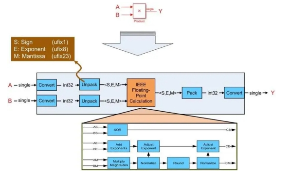
Figure 1 How the hdl encoder maps a single-precision floating-point multiplication to fixed-point hardware resources

The generated vhdl or Viilog logic then performs a floating-point computation (multiplication in the case shown in Figure 1) by calculating the sign bits generated by the input sign bits, the number multiplication, and the exponent required to compute the result and the corresponding normalization. The final stage of the logic packs the sign, exponent, and mantissa back into the floating-point data type.

Solving Dynamic Range Problems with Fixed-Point Conversions

A simple expression, such as (1-A)/(1+A), that needs to be implemented over a high dynamic range can be translated naturally by using single-precision floating-point (Figure 2).

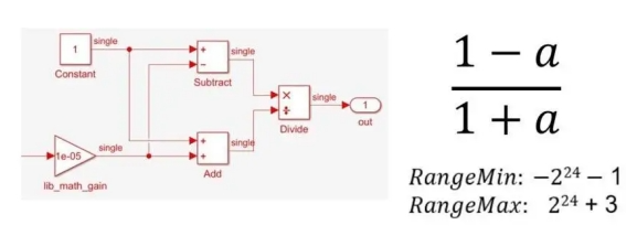
Figure 2. Single-precision implementation of (1-a)/(1+a)

However, implementing the same equation at a fixed-point requires many steps and numerical considerations (Figure 3).

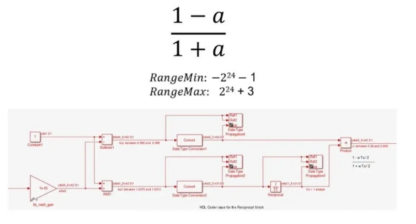
Figure 3. Fixed-point implementation of (1-a)/(1+a)

For example, you must divide division into multiplication and reciprocity, perform nonlinear reciprocal operations using approximation methods such as Newton-Raphson or LUT (look-up table), use different data types to carefully control bit growth, choose appropriate numerator and denominator types, and use specific output types and accumulator types for expansions and subtractions.

Exploring CIR implementation options

Let's look at an example of an infinite impulse response filter. An ir filter requires high dynamic range computation with a feedback loop, making it difficult to converge to a fixed point of quantization. Figure 4A shows a test environment that compares three versions of the same IRR filter with a noisy sine wave input. The amplitude of the sine wave is 1, and the added noise increases the amplitude slightly.

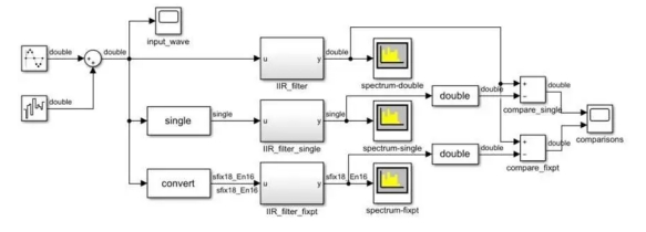
Figure 4A Realization of three ir filters with noisy sine wave inputs.

The first version of the filter is double precision (Figure 4B). The second version is single precision. The third version is a fixed-point realization (Fig. 4C). This implementation results in a data type with up to 22 bits, one of which is assigned to the sign and 21 to the fraction. This particular data type leaves 0 bits to represent integer values, which is reasonable since, given a stimulus, it will always have a value range between -1 and 1. If the design must use different input values, this needs to be taken into account during fixation quantization.

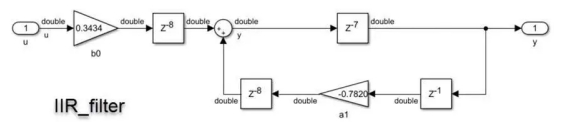
Figure 4B Iir_filter implementation, shown with double exact data type Figure 4c Iir_filter_fixed implementation using fixed-point data type

A test environment was set up to compare the results of the single-precision and fixed-point filters with the double-precision filter, which is considered the golden reference. In both cases, the loss of precision produces some error. The question is whether that error is within the acceptable tolerance of our application.

When we ran Fixed Point Designer to perform the conversion, we specified an error tolerance of 1%. Figure 5 shows the results of the comparison. The single precision version has an error of around 10. -8 , while the fixed-point data type has an error of about 10 -5 . This is within our specified error range. If your application requires higher precision, you may want to increase the fixed word length.

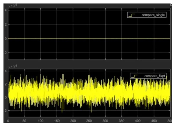
Figure 5 Simulation results comparing double-precision IRR filter results with single-precision results (top) and fixed-point results (bottom).

This kind of quantized fusion requires experience in hardware design, a thorough understanding of possible system inputs, explicit precision requirements, and some help from the fixed-point designer. If this helps to narrow down the algorithm for production deployment, then the effort is worthwhile. But what about situations where simple deployment to prototype hardware is required, or where accuracy requirements make it difficult to reduce the physical footprint? In these cases, one solution is to use single precision local floating point.

Simplifying the Process with Native Floating Point

There are two advantages to using native floating point.

- You don't need to spend time trying to analyze the minimum number of bits required to keep a wide variety of input data accurate enough.

- The dynamic range of single-precision floating-point operations is more efficient at a fixed cost of 32 bits.

Now, the design process is much simpler, and you know that with sign, exponent, and trailing bits, you can represent a wide dynamic range of numbers. The table in Figure 6 compares the floating-point resource utilization using the data type selection shown in Figure 5 with the fixed-point implementation of the ir filter.

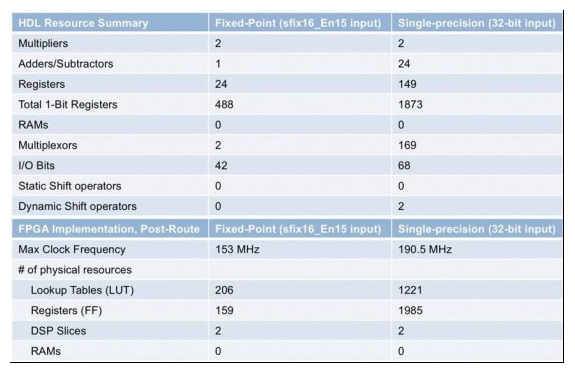
Figure 6 Comparison of resource utilization for fixed-point and floating-point implementations of the ir filter

When you compare the results obtained from the floating-point and fixed-point implementations, keep in mind that floating-point computations require more operations than simple fixed-point algorithms. Using single precision will result in higher physical resource usage when deployed to an FPGA or ASIC. If circuit area is an issue, then you will need to trade off higher precision and resource usage. You can also use a combination of floating-point and fixed-point to reduce area while maintaining single precision to achieve high dynamic range for digitally intensive computations.